Notebook Entry
Reading notes for Modern Particle Physics, Mark Thomson (Chapter 5)
Kind of short notes… Calculations are omitted, maybe update them another time.
Chapter 5 Interaction by particle exchange
First- and second-order perturbation theory
Two perspective for particle interaction:
-
Perspective 1:
The particle goes through a potential field.
-
Perspective 2:
The particle interact with another particle by exchanging particles.
According to the perturbation theory,
\[\Gamma_{fi}= 2\pi |T_{fi}|^2\rho(E_f)\]where
\[T_{fi} = <f|V|i> + \sum_{i\neq j }\frac{<f|V|j><j|V|i>}{E_i-E_j}\]Apparently the 1st term corresponding to the 1st perspective, the 2nd term corresponding to the 2nd perspective. However, the 1st perspective is kind of ‘instantaneous interaction”, which is unreasonable for modern perspective.
Time-ordered perturbation theory
For scattering process $a+b \to c+d$, there’s 2 time order for the simplest process:
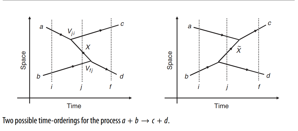
Take the left one for example, we have
\[T_{fi}^{ab} = \frac{<d|V|b+X><c+X|V|a>}{(E_a+E_b)-(E_b+E_c+E_X)}\]Using the relationship between the amplitude V and M, where we take M as the simplest case – the scalar $g_a$, and transform the amplitude T into M, then sum it up, we have
\[M_{fi} = \frac{g_ag_b}{[(E_a-E_c)^2-E_x^2]}\]It’s worth noticing that the process appears at each vertex has momentum conserved (at the cost of plane wave in real space), but not energy conserved(the property of intermediate state).
So far, the particle appears(disappears) at each vertex is still real particle, so it satisfies the mass-energy relation, and we have
\[M_{fi} = \frac{g_ag_b}{q^2-m^2}\]where $q = (E_a-E_c, \vec p_a-\vec p_c)$.
If we consider q as the 4-momentum for the intermediate particle, we can obtain the conservation of energy and momentum at the same time, as the cost of the loss of on-shell condition.
Feynman diagrams and virtual particles
Scattering in a potential
Apparently the interaction of changing particles can be simplified to the potential. For example, the Yukawa potential.
Introduction to QED
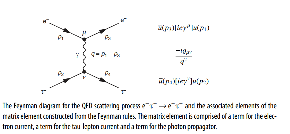
Say a QED process $e^-\tau^-\to e^-\tau^- $to calculate the scalar $g$. In this case, the potential is electromagnetic field which we are familiar with. Use the substitution for electromagnetic interaction, we have
\[H = E+V = (\gamma_0 m - \mathrm i \vec \gamma \cdot \nabla + Q_e\gamma^0\gamma^\mu A_\mu)\]where $A_\mu = \epsilon^{(\lambda)}_\mu\mathrm e^{(\mathrm i \vec p \cdot x -Et)}$ is the vector amplitude for photon, and the index $\lambda$ indicates the polarization for all scenarios(4 in total). .
After considering all cases, we have
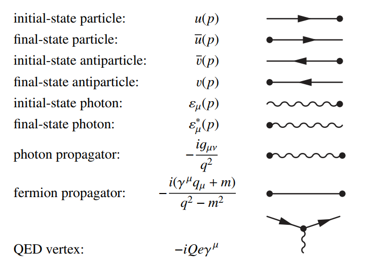
\[M = -[Q_e\bar u_e(p_3)\gamma^\mu u_e(p_1)]\frac{g_{\mu\nu}}{q^2}[Q_\tau e \overline u_\tau(p_4)\gamma^\nu u_\tau(p_2)]\]Feynman rules for QED
We can get the final equation by the composition of Feynman diagram:
Treatment of antiparticles
The first particle encountered when following the line representing a fermion current from the end to the start in the direction against the sense of the arrows, always appears as the adjoint spinor.