Notebook Entry
Reading notes for Modern Particle Physics, Mark Thomson (Chapter 7)
Chapter 7 Electron–proton elastic scattering
Probing the structure of the proton
Four different stages of electron-proton interaction:
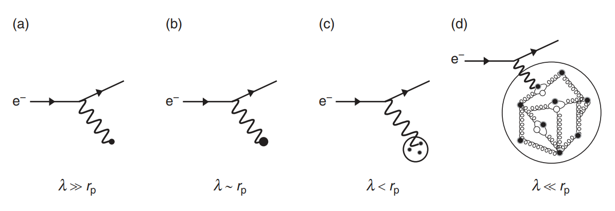
- the electron is far away from the proton, as if the proton is a point positive charge.
- the electron is close to the proton, so the influence of the distribution of charge and the magnetic momentum should be taken into consideration.
- the electron is more closer to the proton, and the electromagnetic interaction with quarks should be taken into account.
- the electron is almost in the proton, so the strong and weak interaction between the electron and quarks should not be neglected.
Rutherford and Mott scattering
Rutherford and Mott scattering are the low-energy limits of e-p elastic scattering.
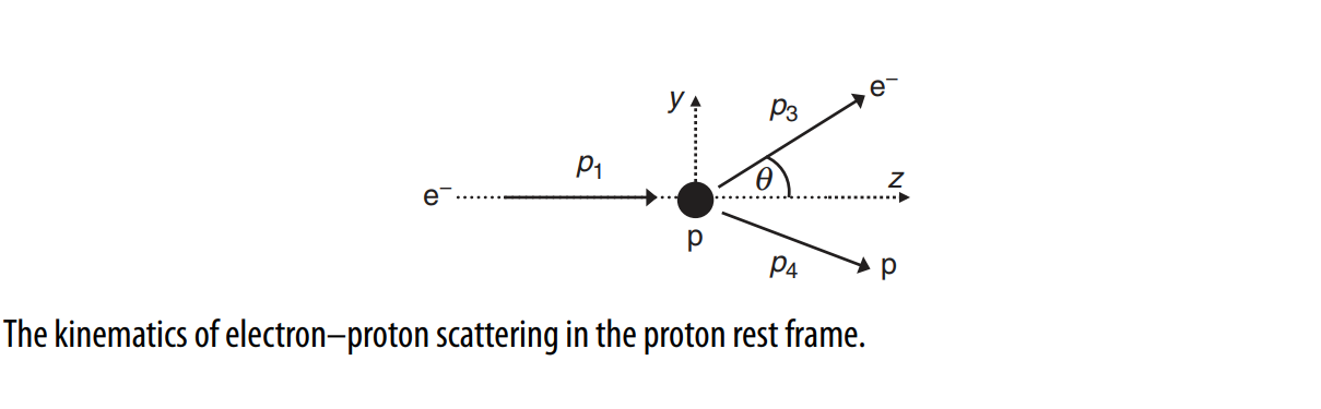
the Feynman diagram for electron-proton elastic scattering:
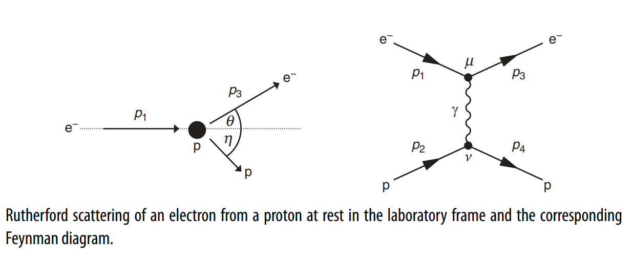
Given $m_e \ll m_p$, the recoil of the proton can be neglected. and $p_1^2 \approx p_3^2$.
According to the angles in the picture above left, we have
Therefore
and
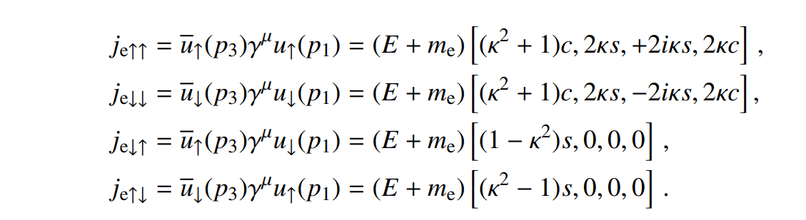
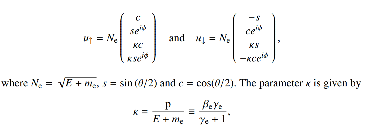
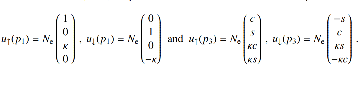
Similar to the calculation of the current of the electron, we have
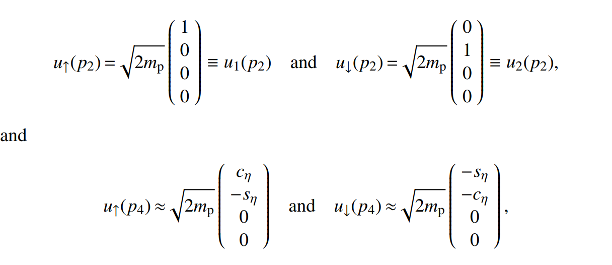
Note that the setting of $c_\eta, s_\eta$ could be arbitrary, since in fact the proton doesn’t move at all.
the current

the average amplitude
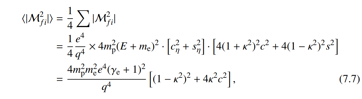
Given that $q = p_1 - p_3= p(0, 1-\cos\theta,-\sin\theta,0)$, we have
\[q^2 = - p^2(1-\cos\theta)^2-p^2\sin^2\theta = -2p^2(1-\cos\theta)=-4p^2\sin^2\frac \theta 2\]Note that in the scattering process, the four-interval $q^2<0$, which don’t bother us since it’s the virtual particle that doesn’t actually exist in real physics.
Finally we get
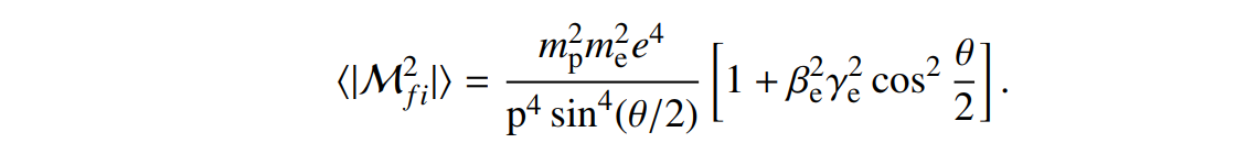
Rutherford scattering
In the limitation of non-realistic situation, we obtain
\[\langle |M_{fi}^2|\rangle = \frac{m_p^2m_e^2e^4}{p^4\sin^4(\frac \theta 2)}\]the differential cross section
\[\frac{\mathrm d \sigma}{\mathrm d \Omega}= \frac{|M_{fi}|^2}{64\pi^2}\frac{1}{(m_p+E_1-E_1\cos\theta)^2}\approx \frac{\alpha^2}{16 E_k^2\sin^4(\frac \theta 2)}\]This result are perfectly aligned with the classical Rutherford scattering results!
Mott scattering
In the limitation of extra-realistic situation (still negligible to the mass of the proton), we obtain
\[\langle |M_{fi}^2|\rangle = \frac{m_p^2e^4}{p^2\sin^4(\frac \theta 2)}\cos^2(\frac\theta 2)\] \[\frac{\mathrm d \sigma}{\mathrm d \Omega}= \frac{|M_{fi}|^2}{64\pi^2}\frac{1}{(m_p+E_1-E_1\cos\theta)^2}\approx \frac{\alpha^2}{4 E_k^2\sin^4(\frac \theta 2)}\cos^2(\frac \theta 2)\]Form factors
Let’s calculate this amplitude in a different view:
Suppose the electron travels in the potential $V(\vec r)$. With the Coulomb’s law, we have
\[V(\vec r)= \frac 1 {4\pi}\int \frac{\rho(\vec r^\prime)}{|\vec r -\vec r ^\prime|}\mathrm d \vec r^\prime\]And
\[M_{fi}= \bra {\psi_f}V(\vec r)\ket {\psi_i} = \int \mathrm d \vec r\mathrm e ^{-\mathrm i \vec p_3 \cdot \vec r}\cdot \frac 1 {4\pi}\int \frac{\rho(\vec r^\prime)}{|\vec r -\vec r ^\prime|}\mathrm d \vec r^\prime\mathrm e ^{\mathrm i \vec p_1 \cdot \vec r}=\frac{1}{4\pi}\int \frac{\mathrm e^{\mathrm i \vec q\cdot \vec R}}{|\vec R|}\mathrm d \vec R \int \rho(\vec r^\prime)\mathrm e^{\mathrm i \vec q \cdot \vec r^\prime}\mathrm d \vec r^\prime= M_{fi}^{pt}F(\vec q^2)\]where $F(\vec q^2)$ called form factor.
Relativistic electron–proton elastic scattering
For more precise calculation, let’s add the recoil of the proton back.
where
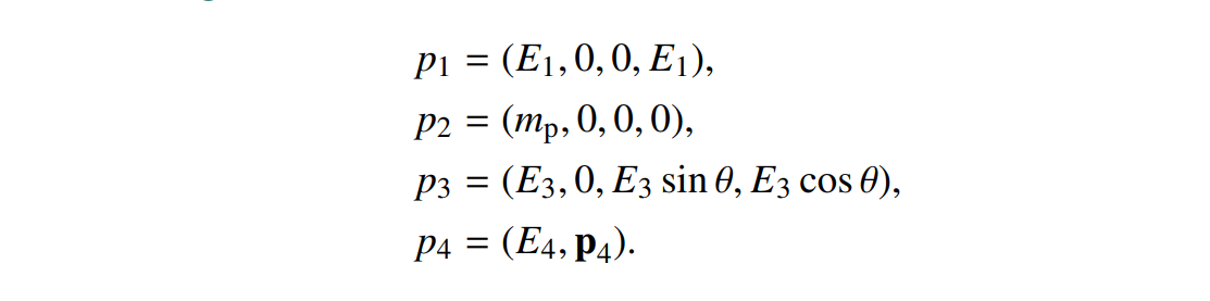
Thus
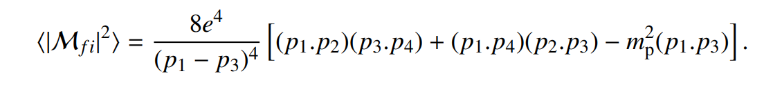
According to the equations above, we obtain
\[\langle |M_{fi}^2|\rangle =\frac{m_pe^4}{E_1E_3\sin^4 (\frac \theta 2)}((E_1-E_3)\sin^2\frac \theta 2+m_p\cos^2\frac \theta 2)\]With
\[q^2 = -2E_1E_3(1-\cos \theta)\]always negative, we define
\[Q^2 = -q^2 = 2m_p\cdot (E_1-E_3)\]the last equality is not that obvious …
To demonstrate a reasonable way to calculate this: \(\begin{aligned} m_p^2 = p_4^2 &= (p_1+p_2-p_3)^2 \\ &= p_1^2+p_2^2+p_3^3+2p_1\cdot p_2-2p_1\cdot p_3- 2p_2\cdot p_3\\ &= m_p^2+2E_1m_p-2E_1E_3(1-\cos\theta)-2m_pE_3 \end{aligned}\)
thus
\[\langle |M_{fi}^2|\rangle =\frac{m_p^2e^4}{E_1E_3\sin^4 (\frac \theta 2)}(\frac{Q^2}{2m_p^2}\sin^2\frac \theta 2+\cos^2\frac \theta 2)\]Apparently the term
\[E_3 = \frac{m_pE_1}{m_p+E_1(1-\cos\theta)}\] \[Q^2 =\frac{2m_pE_1E_3(1-\cos\theta)}{m_p+E_1(1-\cos\theta)}\]The Rosenbluth formula
Further more, consider the distribution of the charge of the proton and the magnetic momentum of the proton, we have the Rosenbluth formula:
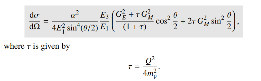
for the proton,
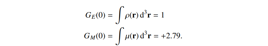
Some discussions for this formula:
Measuring $G_E(Q^2)$ and $G_M(Q^2)$
Define (the result of Mott scattering)
\[\left(\frac{\mathrm d \sigma}{\mathrm d \Omega}\right)_0 =\frac{\alpha^2}{4 E_1^2\sin^4(\frac \theta 2)}\frac{E_3}{E_1}\cos^2(\frac \theta 2)\]we have
\[\frac{\mathrm d \sigma}{\mathrm d \Omega} = \left(\frac{\mathrm d \sigma}{\mathrm d \Omega}\right)_0\cdot \left(\frac{G_E^2+\tau G_M^2}{1+\tau}+2\tau G_M^2\tan^2\frac\theta 2\right)\]when $\tau \ll 1$,
\[\frac{\mathrm d \sigma}{\mathrm d \Omega} = \left(\frac{\mathrm d \sigma}{\mathrm d \Omega}\right)_0 G_E^2\]just the result for Mott scattering. When $\tau \gg 1$,
\[\frac{\mathrm d \sigma}{\mathrm d \Omega} = \left(\frac{\mathrm d \sigma}{\mathrm d \Omega}\right)_0\cdot \left(1+\tau \tan^2\frac\theta 2\right)G_M^2\]Elastic scattering at high $Q^2$
Just the equation above with 1 in the left side omitted.